A Road Map of Nonparametric Efficiency in Causal Inference

Causal inference promises to answer “what if” questions from observational data. But the standard approach — specify a parametric model, fit it, report the estimate — breaks down under misspecification. And misspecification is the norm, not the exception. This post draws from my notes on (Kennedy 2023). I walk through the core ideas of nonparametric efficiency theory — the framework that lets us pair flexible machine learning with rigorous inference. The central character is the Efficient Influence Function, a single mathematical object that tells us how to build estimators, why they work, and when we can trust their confidence intervals.

1. Motivation

First let’s keep the casual and statistical issues separate.

Causal to Statistical: The target causal parameter (e.g., ATE) can often be identified as a statistical functional of the observed data distribution.

$$\psi: \mathcal{P} \mapsto \mathbb{R}$$

Once identified, the causal problem becomes a pure functional estimation problem.

The Problem with Parametrics: Parametric models are likely misspecified, leading to biased estimates of the functional.

The Problem with Naive Nonparametrics: While we should use flexible machine learning (nonparametric) methods to avoid misspecification, simple “plug-in” estimators (fitting models and plugging predictions into the formula) fail because:

• They are generally not $\sqrt{n}$-consistent (converge too slowly).

• They do not yield valid Confidence Intervals.

The Solution: We need Efficiency Theory to understand the theoretical limit of performance and Influence Functions to construct estimators that reach that limit.

2. Efficiency Theory (Lower Bounds)

Now let’s build the “best” estimator.

The Benchmark: We want to find the best possible performance (lowest Mean Squared Error) any estimator can achieve.

Parametric Intuition: In parametric models, the Cramer-Rao (CR) lower bound sets this benchmark: no unbiased estimator can have a variance lower than the inverse Fisher information.

But now we are in the “nonparametric world”, how to exploit CR lower bound?

The “Submodel” Trick: To apply CR bounds to infinite-dimensional nonparametric models:

• We define a Parametric Submodel: a smooth, one-dimensional path through the complex nonparametric space that passes through the true distribution.

• Logic: If we cannot estimate the parameter well in this simple “parametric” slice, we certainly cannot do it in the full nonparametric model.

• Result: The hardest submodel defines the Local Minimax Lower Bound.

3. The Unified Approach: Central Role of the EIF

The Efficient Influence Function (EIF) is the “master key.” It is the derivative term in a Distributional Taylor Expansion¹ (von Mises expansion):

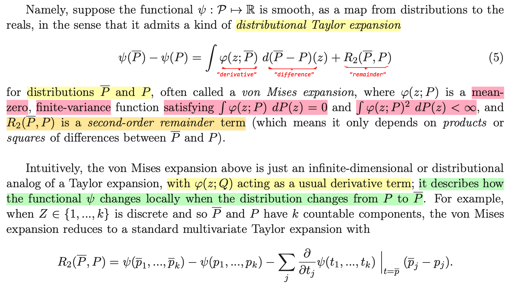
This single expansion solves all three statistical tasks:

A. How to construct the estimator? (The Recipe)

The expansion reveals that the bias of a naive plug-in estimator is roughly the expected value of the EIF.

Recipe: We construct a One-Step Estimator by taking the naive plug-in estimator and adding the empirical average of the estimated EIF to “de-bias” it.

$$ \hat{\psi}_{\text{one-step}} = \text{Plug-in} + \frac{1}{n}\sum \text{EIF}(\text{Data}) $$

B. How to analyze the estimator? (The Proof)

The expansion includes a Remainder Term ($R_2$). To prove the estimator is $\sqrt{n}$-consistent, we must show this remainder is negligible (second-order).

Sample Splitting: We need to use cross-fitting to handle the “empirical process term” (preventing overfitting when estimating nuisance parameters).

C. How to correct the bias? (Double Robustness)

The math of the EIF reveals that the error depends on the product of errors of the nuisance parameters (e.g., error in outcome regression $\times$ error in propensity score).

This yields Double Robustness: even if individual machine learning models converge slowly (e.g., $n^{-1/4}$), their product converges fast enough ($n^{-1/2}$) to allow for valid inference.

4. The Link Between EIF and Riesz Representer

The connection between the Efficient Influence Function (EIF) and the Riesz Representer (RR) is the bridge between theoretical statistics and practical machine learning.

The Deconstruction of the EIF

We already know the EIF is the “correction term” we add to a naive plug-in estimator to fix bias. The Riesz Representer is the key component inside that EIF.

For a vast class of problems (linear functionals), the EIF always takes this specific structure:

• $\mu(X, W)$: The conditional expectation (the outcome model, e.g., regression of $Y$ on $X, W$).

• $\alpha(X, W)$: The Riesz Representer. It tells us how much weight to give each residual to correct the bias.

• The EIF says: “To fix bias, look at your regression errors ($Y - \mu$).”

• The RR says: “Here is exactly how to weight those errors for this specific causal problem.”

Takeway

Here is the takeaway. Nonparametric efficiency theory is not an abstraction separate from practice — it is the practice. The EIF tells us what to estimate, the Riesz Representer tells us how to weight the errors, and double robustness explains why the whole thing holds together even when our models are imperfect. If we use AIPW, DML, or any doubly robust estimator, we are already using these ideas. The theory simply makes explicit what those estimators are doing and why they deserve our trust.

Reference

Kennedy, Edward H. (2023), “Semiparametric doubly robust targeted double machine learning: a review.”

Williams, Nicholas T., Oliver J. Hines, and Kara E. Rudolph (2026), “Riesz representers for the rest of us.”

Chernozhukov, Victor, Whitney K. Newey, Victor Quintas-Martinez, and Vasilis Syrgkanis (2024), “Automatic debiased machine learning via riesz regression.”

Chernozhukov, Victor, Whitney K. Newey, and Rahul Singh (2022), “Automatic Debiased Machine Learning of Causal and Structural Effects,” Econometrica, 90 (3), 967–1027.