Notes on Causal Survival Forest 🌲⏳
In this post, I provide summary notes on the paper “Estimating Heterogeneous Treatment Effects with Right-Censored Data via Causal Survival Forests” by Cui et al. (2023).
Motivation
How to estimate heterogeneous treatment effects with right-censored data?
-
Heterogeneous treatment effect (HTE) estimation plays a central role in data-driven personalization
-
Existing methods often can’t handle censored survival outcomes, common in medical/business applications
Causal Survival Forests (CSF)
To address this challenge, the paper proposes causal survival forests (CSF)

-
An adaptation of the causal forest algorithm of Athey et al. (2019)
-
It adjusts for censoring using doubly robust estimating equations developed in the survival analysis literature
Advantages
-
Doubly robust, computationally tractable, and outperforms available baselines in our experiments
-
Good statistical properties – UCAN
Setting and notation
Assume i.i.d tuples $\{X_i, T_i, C_i, W_i\}$, where
- $X_i \in \mathcal{X}$ denote covariates
- $T_i \in \mathbb{R}_{+}$ is the survival time for $i$th unit
- $C_i \in \mathbb{R}_{+}$ is the censoring time (the time at which $i$th unit gets censored)
- $W_i \in \{0,1\}$ denotes a binary treatment
Using potential outcome framework, posit potential outcomes $\{T_i(1), T_i(0)\}$ s.t. $T_i = T_i(W_i)$, we need to estimate the conditional average treatment effect (CATE)
$$ \tau(x)=\mathbb{E}\left[y(T_i(1)) - y(T_i(0)) \mid X_i=x\right], $$
where $y()$ is the outcome transformation. For example,
-
$y(T) = T$
-
$y(T) = T \wedge h$ for the restricted mean survival time (RMST); here $h$ is some chosen maximum considered time
-
$y(T) = \1\{T \ge h\}$ for the survival probability
To estimate $\tau(x)$, the main challenge is that $T_i$ is not always observable. We can only observe:
-
censored survival time: $U_i = T_i \wedge C_i$
-
non-censoring indictor: $\Delta_i = 1\{T_i \le C_i\}$
Based on Assumption 1 (see later), we define the effective non-censoring indictor as follows:
\begin{align} \Delta_i^h &= 1\{T_i \wedge h \le C_i\} \\ &\overset{(2)}{=} \Delta_i \vee 1\{U_i \ge h\} \end{align}Note that, for the eqn (2), everything is observed. We can regard an observation with $\Delta_i^h = 1$ as a complete observation.
Assumptions
In order to identify treatment effects, we need to rely on two sets of assumptions.
-
Assumption 2-4 enable us to identify the causal effect of $W_i$ on $T_i$ without censoring
-
Assumption 5-6 is to guarantee that censoring due to $C_i$ does not break identification results
Assumption 1 (Finite Horizon)
$$ y(t) = y(h), \quad \forall \ t \ge h, \ 0<h<\infty $$
Assumption 2 (Potential Outcomes)
$$ \{T_i(1), T_i(0)\} \quad s.t. \quad T_i = T_i(W_i) \quad a.s. $$ Assumption 3 (Ignorability)
$$ \{T_i(1), T_i(0)\} \perp W_i \mid X_i $$Assumption 4 (Overlap)
Propensity score $e(x) = \mathbb{P}(W_i = 1\mid X_i = x)$ is uniformly bounded away from 0 and 1,
$$ \eta_e \le e(x)\le 1- \eta_e, \quad 0< \eta_e \le \frac{1}{2} $$
Assumption 5 (Ignorable censoring)
Censoring is independent of survival time conditionally on treatment and covariates,
$$ T_i \perp C_i \mid W_i, X_i $$
Assumption 6 (Positivity)
$$ \mathbb{P}(C_i < h | W_i, X_i) \le 1- \eta_c, \quad 0<\eta_c\le1 $$
Causal Forests Without Censoring
How does causal forest work?
Essentially, we are running a “forest”-localized version of Robinson’s regression
$$ \tau(x):=\operatorname{lm}\left(Y_i-\hat{m}^{(-i)}\left(X_i\right) \sim W_i-\hat{e}^{(-i)}\left(X_i\right), \text { weights }=\textcolor{blue}{\alpha_i(x)}\right), $$
where
-
$\textcolor{blue}{\alpha_i(x)}$ capture how “similar” a target sample $x$ is to each of the training samples $X_i$
-
$\hat{m}$ and $\hat{e}$ are machine learning estimates for the outcome and propensity score models with cross-fitting
Using notations in previous section, we estimate $\tau(x)$ by solving the following equation,
$$ \sum_{i=1}^n \alpha_i(x) \psi_{\hat{\tau}(x)}^{(c)}\left(X_i, y\left(T_i\right), W_i ; \hat{e}, \hat{m}\right)=0 \tag{cf} $$
where,
\begin{aligned} \psi_\tau^{(c)}\left(X_i, y\left(T_i\right), W_i ; \hat{e}, \hat{m}\right) &= \left[ W_i - \hat{e}\left(X_i\right) \right] \quad \times\\ & \left[ y\left(T_i\right) - \hat{m}\left(X_i\right) - \tau \left( W_i - \hat{e}\left(X_i\right) \right) \right] \end{aligned}is the orthogonal complete score function (shown as up-script $^{(c)}$),
-
$e(x) = \mathbb{P}(W_i = 1\mid X_i = x)$
-
$m(x) = \mathbb{E}(y(T_i) \mid X_i)$
-
$\hat{e}(X_i)$ and $\hat{m}(X_i)$ are estimates derived via cross-fitting
Adjusting for Censoring via Weighting
In the presence of censoring, the $T_i$ in equation (cf) is no longer observable.
Simply ignoring censoring and building models on with complete observations (i.e. $\Delta_i^h = 1$) would lead to bias.
Simple Censoring Adjustment via IPCW
Define the conditional survival function for censoring process as $$ S_w^C(s \mid x)=\mathbb{P}\left[C_i \geq s \mid W_i=w, X_i=x\right] $$ We have, $$ \mathbb{P}\left[\Delta_i^h=1 \mid X_i, W_i, T_i\right]=S_{W_i}^C\left(T_i \wedge h \mid X_i\right) $$
-
the LHS is the conditional probability of observing a complete observations (i.e. $\Delta_i^h = 1$)
-
the RHS is the conditional probability that censoring time is greater than survival time
-
Does the above $\mathbb{P}(\Delta_i^h = 1 \mid \cdots)$ look like propensity score function?
The main idea of IPCW estimation is to only consider complete cases, but up-weight all complete observations by $1/S_{W_i}^C\left(T_i \wedge h \mid X_i\right)$ to compensate for censoring.
As a result, IPCW estimators succeed in eliminating censoring bias.
With IPCW, we estimate $\tau(x)$ by solving the following equation,
$$ \sum_{\left\{i: \Delta_i^h=1\right\}} \frac{\alpha_i(x)}{\hat{S}_{W_i}^C\left(T_i \wedge h \mid X_i\right)} \psi_{\hat{\tau}(x)}^{(c)}\left(X_i, y\left(T_i\right), W_i ; \hat{e}, \hat{m}\right)=0 \tag{IPCW} $$ Let’s compare the equation (cf) v.s (IPCW),
-
For eqn (cf), we sum over all observations; for eqn (IPCW), we only sum over complete observations
-
For eqn (IPCW), we add $\frac{1}{1/S_{W_i}^C\left(T_i \wedge h \mid X_i\right)}$ as a part of weight
For more details on IPCW, please check:
-
Chapter 8 and 12 in the textbook Causal Inference: What If" (Hernán and Robins, 2020). In particular, “Ch 12.6 Censoring and missing data” is very helpful.
-
Chapter 21 “Treatment Heterogeneity with Survival Outcomes” in the textbook Handbook of Matching and Weighting Adjustments for Causal Inference (Zubizarreta et al., 2023)
A Doubly Robust Correction
Two limitations of IPCW approach:
-
Only use complete observations; throw away all observations with $\Delta_i^h = 0$, and this may hurt efficiency
-
IPCW-type methods are generally not robust to estimation errors; Neyman orthogonality condition (Chernozhukov et al. 2018) does not hold
CSF Method
CSF method does not rely on IPCW. Instead, it relies on a more robust approach to making estimating equations robust to censoring.
Recall the simplest case (without censoring), we have,
$$ \sum_{i=1}^n \alpha_i(x) \psi_{\hat{\tau}(x)}^{(c)}\left(X_i, y\left(T_i\right), W_i ; \hat{e}, \hat{m}\right)=0 \tag{cf} $$
where
- $\psi_{\hat{\tau}(x)}^{(c)} (\cdot)$ is the score function with the complete data
The idea of CSF is to convert the above (cf) equation into a censoring robust estimating equation by using estimates of the survival and censoring processes.
Now, we estimate the $\tau(x)$ by solving the following equation,
$$ \sum_{i=1}^n \alpha_i(x) \psi_{\hat{\tau}(x)}\left(X_i, y\left(U_i\right), U_i \wedge h, W_i, \Delta_i^h ; \hat{e}, \hat{m}, \hat{\lambda}_w^C, \hat{S}_w^C, \hat{Q}_w\right)=0, $$where the score function is,
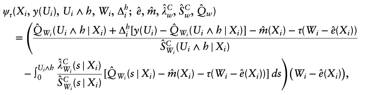
the conditional expectation of the transformed survival time is defined as:
$$ Q_w(s \mid x)=\mathbb{E}\left[y\left(T_i\right) \mid X_i=x, W_i=w, T_i \wedge h>s\right] $$
and the associated conditional hazard function is defined as:
$$ \lambda_w^{\mathrm{C}}(s \mid x)=-\frac{d}{d s} \log S_w^{\mathrm{C}}(s \mid x) $$
$\hat{Q}_w(s \mid x), \hat{S}_w^C(s \mid x)$ and $\hat{\lambda}_w^C(s \mid x)$ are cross-fit nuisance parameter estimates.
How to understand the above score function?The short answer is that that functional form emerges for the math (i.e., the desire for a doubly robust adjustment); and, unlike with the basic AIPW formula, it’s not as immediately intuitive.1
💡 KEY Points
We should think about the Neyman-orthogonal property. In summary, CSF alleviates the drawbacks of IPCW so by taking the (complete-data) causal forest estimating equation $\psi_{\tau(x)}^{(c)}(T, W, \ldots)$ (the “R-learner”) and turn it into a censoring robust estimating equation $\psi_{\tau(x)}(Y, W, \ldots)$ by using estimates of the survival and censoring processes2. ("…" refers to additional nuisance parameters):
-
censoring process: $P\left[C_i>t \mid X_i=x, W_i=w\right]$
-
survival process: $P\left[T_i>t \mid X_i=x, W_i=w\right]$
The upshot of this “orthogonal” estimating equation is that it will be consistent if either the survival or censoring process is correctly specified, which is very beneficial when we want to estimate these by modern ML tools, such as random survival forests.
For more details, Rubin & van der Laan (2007) and the chapter on RCTs with time-to-event data in Targeted Learning (2011) gives some more digestible details on doubly robust estimation with survival data.3
I also found the code in grf GitHub repo helpful to understand the implement procedure. Specifically, check the following lines:
# The conditional survival function for the survival process.
sf.survival <- do.call(grf::survival_forest, c(list(X = cbind(X, W), Y = Y, D = D), args.nuisance))

# The conditional survival function for the censoring process.
sf.censor <- do.call(grf::survival_forest, c(list(X = cbind(X, W), Y = Y, D = 1 - D), args.nuisance))
References
Athey, Susan, Julie Tibshirani, and Stefan Wager. 2019. “Generalized Random Forests.” The Annals of Statistics 47 (2): 1148–78. https://doi.org/10.1214/18-AOS1709.
Chernozhukov, Victor, Denis Chetverikov, Mert Demirer, Esther Duflo, Christian Hansen, Whitney Newey, and James Robins. 2018. “Double/Debiased Machine Learning for Treatment and Structural Parameters.” The Econometrics Journal 21 (1): C1–68. https://doi.org/10.1111/ectj.12097.
Cui, Yifan, Michael R Kosorok, Erik Sverdrup, Stefan Wager, and Ruoqing Zhu. 2023. “Estimating Heterogeneous Treatment Effects with Right-Censored Data via Causal Survival Forests.” Journal of the Royal Statistical Society Series B: Statistical Methodology 85 (2): 179–211. https://doi.org/10.1093/jrsssb/qkac001.
Hernán MA, Robins JM (2020). Causal Inference: What If. Boca Raton: Chapman & Hall/CRC.
Zubizarreta, J. R., Stuart, E. A., Small, D. S., & Rosenbaum, P. R. (2023). Handbook of Matching and Weighting Adjustments for Causal Inference. CRC Press.
-
This was suggested by Professor Wager in an email conversation. ↩︎
-
Check more on grf tutorial: Causal forest with time-to-event data ↩︎
-
Suggested by Erik Sverdrup. Many thanks! ↩︎