Study Notes on Bounding OVB 🌀 in Causal ML
Motivation
In empirical research, one of the challenges to causal inference is the potential presence of unobserved confounding. Even when we adjust for a wide range of observed covariates, there’s often a lingering concern: what if there are important variables we’ve failed to measure or include? This challenge necessitates a careful approach to sensitivity analysis, where we assess how strong unobserved confounders would need to be to meaningfully alter our conclusions.

Questions1
-
How “strong” would a particular confounder (or group of confounders) have to be to change the conclusions of a study?
-
In a worst case scenario how vulnerable is the study’s result to many or all unobserved confounders acting together, possibly nonlinearly?
-
Are these confounders or scenarios plausible? How strong would they have to be relative to observed covariates (e.g female), in order to be problematic?
-
How can we present these sensitivity results concisely for easy routine reporting?
TL;DR
Chernozhukov et al. (2024) introduces a framework for bounding omitted variable bias (OVB) in causal machine learning setting. They develop a general theory applicable to a broad class of causal parameters that can be expressed as linear functionals of the conditional expectation function. The key insight is to characterize the bias using the Riesz representation. Specifically, they express the OVB as the covariance of two error terms:
-
The error in the outcome regression
-
The error in the Riesz representer (RR)
This formulation leads to a bound on the squared bias that is the product of two terms:
- The MSE of the outcome regression
- The MSE of the RR
Theoretical Details
Recall that:
For classical linear regression, “Short equals long plus the effect of omitted times the regression of omitted on included.”
– Angrist and Pischke, Mostly Harmless Econometrics.
In Linear Regression Setting
-
Linear model: $$ Y_i = \alpha + \beta D_i + \gamma^{\intercal} X_i + \delta U_i + \epsilon_i, $$ where $U_i$ is an unobserved (scalar) confounding. Note that, if there are multiple confounders, we can regard $U_i$ as a function of them, which are summarized as a single confounder.
-
Recall the omitted variable bias formula: $$ \hat{\beta} \overset{p}{\rightarrow} \beta + \delta \times \frac{\mathrm{Cov}(U_i^{\perp X}, D_i^{\perp X})}{\mathbb{V}(D_i^{\perp X})}, $$
where
- $D_i^{\perp X} = D_i - \mathrm{lm}(D\sim X)$ is the residual term
- $U_i^{\perp X}$ is the residual from $\mathrm{lm}(U\sim X)$
- $\frac{\mathrm{Cov}(U_i^{\perp X}, D_i^{\perp X})}{\mathbb{V}(D_i^{\perp X})}$ is the coefficient of residual-on-residual regression. It means how much variation of $U$ can be explained by $D$ condition on $X$. In other words, the association between $U$ and $D$ condition on $X$
- $\delta$ is the association between $Y$ and $U$ condition on $\{D, X\}$
-
How to bound the bias?
-
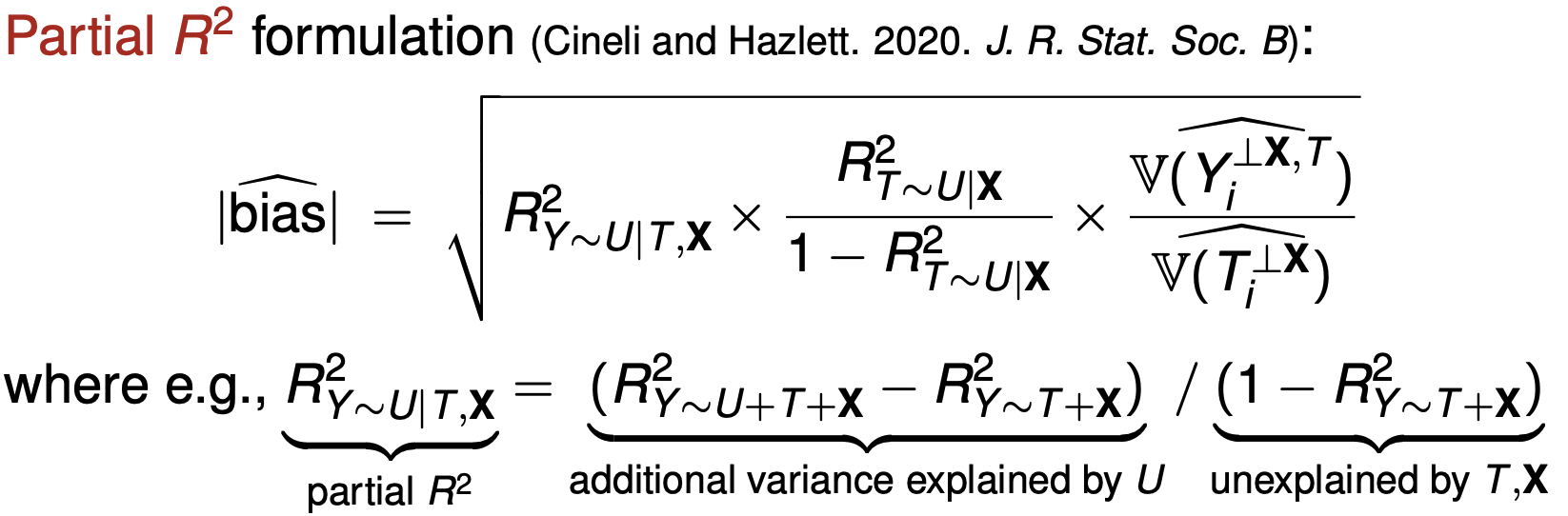
- Partial $R^2$ represents how much variation of $Y$ can explained by $U$ condition on $\{T, X\}$
-
In Causal ML Setting
-
In the ideal case:
-
“long” regression: $Y = \theta D + f(X, A) + \epsilon$
-
Define $W := (D, X, A)$ as the “long” list of regressors
-
$A$ is unobserved vector of covariates
-
Assume $\mathbb{E}(\epsilon \mid D, X, A) = 0$
-
-
In the practical case:
- “short” regression: $Y = \theta_sD + f_s(X) + \epsilon_s$
- Define $W_s := (D,X)$ as the “short” list of observed regressors because $A$ is unmeasured/unobservable
- Use $\theta_s$ to approximate $\theta$; need to bound $\theta_s - \theta$
-
Conditional Expectation (outcome regression function)
-
“long” CET, $g(W) := \mathbb{E}(Y \mid D, X, A) = \theta D + f(X, A)$
-
“short” CET, $g_s(W) := \theta_s D + f_s(X)$
-
-
Riesz Representers (RR):
-
“long” RR: $$ \alpha:= \alpha(W):=\frac{D-\mathrm{E}[D \mid X, A]}{\mathrm{E}(D-\mathrm{E}[D \mid X, A])^2} $$
By FWL Theorem, we have $$ \theta = \frac{Cov(Y\tilde{D})}{Var(\tilde{D})} = \mathbb{E}(y\alpha), \ \text{where } \tilde{D} = D-\mathrm{E}[D \mid X, A], $$
-
“short” RR $$ \alpha_s := \alpha_s\left(W^S\right):=\frac{D-\mathrm{E}[D \mid X]}{\mathrm{E}(D-\mathrm{E}[D \mid X])^2} $$
-
In special case, one can show: $$ \alpha(W)=\frac{D}{P(D=1 \mid X, A)}-\frac{1-D}{P(D=0 \mid X, A)}, $$
$$ \alpha_s(W)=\frac{D}{P(D=1 \mid X)}-\frac{1-D}{P(D=0 \mid X)}, $$
The RR “looks like” the weights in Inverse Propensity Score weighting (IPW). For example,
$$ \begin{aligned} \alpha_s(W) &= \frac{D}{P(D=1 \mid X)}-\frac{1-D}{P(D=0 \mid X)} \\& = \frac{D}{e(X)} - \frac{1-D}{1-e(X)}, \ \, \text{where } e(X) = P(D=1 \mid X) \end{aligned} $$Recall the property of IPW estimator, we have:
$$ \theta_s \overset{ipw}{=} \mathbb{E}\left[\frac{YD}{e(X)} - \frac{Y(1-D)}{1-e(X)}\right] = \mathbb{E}(Y\alpha_s) $$ -
-
Note that, $\theta = \mathbb{E}(g \alpha)$. Why? $$ \begin{aligned} \mathbb{E}(g \alpha) & = \mathbb{E}\left\{ \mathbb{E}(Y \mid D, X, A) \frac{D-\mathrm{E}[D \mid X, A]}{\mathrm{E}(D-\mathrm{E}[D \mid X, A])^2} \right\} \\ &= \mathbb{E}\left\{ [\theta D + f(X, A)] \frac{D-\mathrm{E}[D \mid X, A]}{\mathrm{E}(D-\mathrm{E}[D \mid X, A])^2} \right\} \\ &= \theta \end{aligned} $$
For the third equation, we use the fact that: $\mathrm{E}[D \mid X, A] \ {\perp \!\!\! \perp} \ D-\mathrm{E}[D \mid X, A]$ and $f(X, A) \ {\perp \!\!\! \perp} \ D-\mathrm{E}[D \mid X, A]$.
Short Summary:
-
$g$ is the outcome regression function
-
$\alpha$ is the Riesz Representer
-
We have $\theta = \mathbb{E}(Y\alpha) = \mathbb{E}(g \alpha)$ and $\theta_s = \mathbb{E}(Y\alpha_s) = \mathbb{E}(g_s \alpha_s)$.
Key Results
Key observation:
-
OVB is bounded by $\mathbb{E}(\text{outcome regression error} \cdot \text{RR error})$
-
Square bias is bounded by $\text{MSE(regression)} \cdot \text{MSE(RR)}$
Idea of Proof:
-
Write $\theta = \mathbb{E}(g \alpha)$ and $\theta_s = \mathbb{E}(g_s \alpha_s)$
-
Use the fact that $\alpha_s \ {\perp \!\!\! \perp} \ g-g_s$ and $g_s \ {\perp \!\!\! \perp} \ \alpha - \alpha_s$
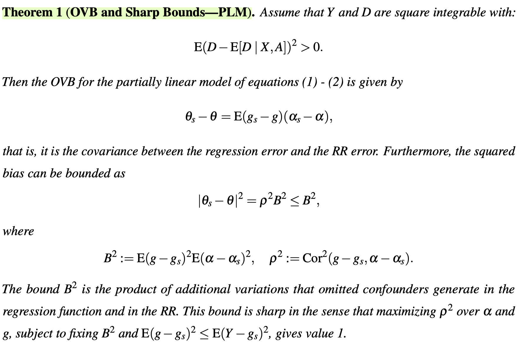
Now, we know the omitted variable bias,
$$\theta_s - \theta = \mathbb{E}(g_s - g)(\alpha_s - \alpha),$$
is the covariance between the regression error,
$$g_s - g = \mathbb{E}(Y|W_s) - \mathbb{E}(Y|W),$$
and RR error,
$$\alpha_s - \alpha,$$
that is, the “weights in IPW” calculated using the short list of regressors, minus the “weights in IPW” using the long list of regressors.
As we can see, this is not easy to interpret, so the following Corollary provides a more intuitive understanding using the familiar $R^2$.
Note that,

The bias is thus bounded by the additional variation that omitted variables cause in the regression function and Riezs representers.
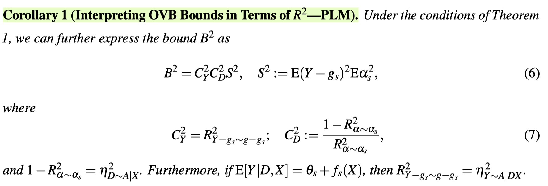
We can make this easier to interpret with further algebra,

Short Summary:
-
$S$ is the scale of the bias, which can be identified from the observed data.
-
The confounding strength $C_Y$ and $C_D$ have to be restricted by the analyst.
-
$C_{Y}^2$ measures the proportion of residual variation of the outcome explained by latent confounders; in short, the strength of unmeasured confounding in outcome equation
-
$C_{D}^2$ measures the proportion of residual variation of the treatment explained by latent confounders; in short, the strength of unmeasured confounding in treatment equation

Empirical Challenge
How do we determine the plausible strength of these unobserved confounders?
This is a critical question, as setting these values arbitrarily could lead to overly conservative or overly optimistic interpretations of our results. We need a principled approach to guide our choices.
Benchmarking
One solution is benchmarking. This approach leverages the observed data to inform our judgments about unobserved confounders. The basic idea is the following: we can use the impact of observed covariates as a reference point for the potential impact of unobserved ones. For instance, if we’ve measured income, the “most” important factor, and found it explains 15% of the variation in our outcome, we might reason that an unobserved confounder is unlikely to have an even larger effect.
In practice, benchmarking can take several forms. We might purposely omit a known important covariate, refit our model, and observe the change. This gives us a concrete example of how omitting an important variable affects our estimates. Alternatively, we could express the strength of unobserved confounders relative to observed ones. For example, we might consider scenarios where an unobserved confounder is as strong as income, or perhaps 25% as strong.
Recent research (Chernozhukov et al.,2024) has demonstrated the utility of this approach. In a study on 401(k) eligibility, they used the observed impact of income, IRA participation, and two-earner status as benchmarks for potential unobserved firm characteristics. Similarly, in a study on gasoline demand, the known impact of income brackets informed the choice of sensitivity parameters for potential remnant income effects.
Robustness Value
Another useful concept is the Robustness Value (RV) which represents the minimum strength of confounding required to change a study’s conclusions. This provides a clear threshold for evaluating the robustness of results.
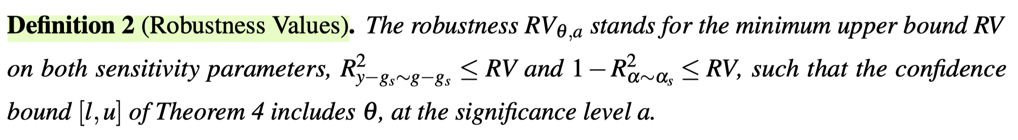
The idea of robustness values is to quickly communicate how robust the short estimate is to systematic errors due to residual confounding. For example, $RV_{\theta = 0, \alpha = 0.05}$ measures the minimal strength on both confounding factors such that the estimated confidence bound for the ATE would include zero, at the 5% significance level.
401(k) example in the paper
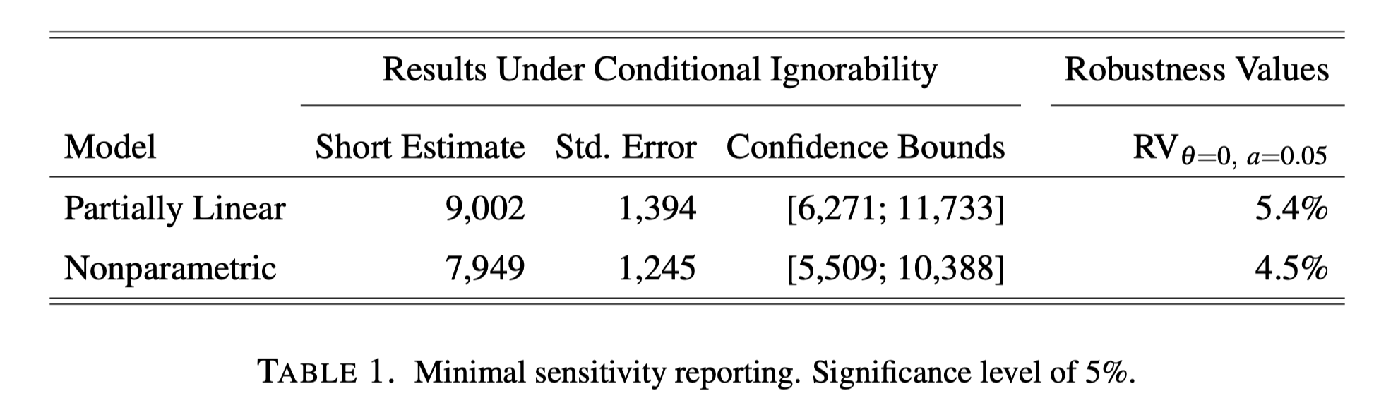
“Table 1 illustrates our proposal for a minimal sensitivity reporting of causal effect estimates. Beyond the usual estimates under the assumption of conditional ignorability, it reports the robustness values of the short estimate.
Starting with the PLM, the $RV_{\theta = 0, \alpha = 0.05} = 5.4 \%$ means that unobserved confounders that explain less than 5.4% of the residual variation, both of the treatment, and of the outcome, are not sufficiently strong to bring the lower limit of the confidence bound to zero, at the 5% significance level.”
Interpretation of RV:
-
A higher RV suggests that the causal estimate is more robust to omitted variable bias because stronger confounding would be needed to alter the conclusions.
-
A lower RV suggests that a relatively small amount of confounding could change the conclusions.
In summary, the robustness value (RV) provides a concise way to communicate how sensitive the results of a causal analysis are to potential omitted variable bias. It is the minimum strength of confounding that would be required to change the conclusions. A larger RV indicates a more robust analysis.
Software to Implement
- carloscinelli/dml.sensemakr: Sensitivity analysis tools for causal ML
- useR! 2020: sensemakr: Sensitivity Analysis Tools for OLS (C.Cinelli), regular - YouTube
References
Chernozhukov, Victor, Carlos Cinelli, Whitney Newey, Amit Sharma, and Vasilis Syrgkanis. “Long Story Short: Omitted Variable Bias in Causal Machine Learning.” arXiv, May 26, 2024. https://doi.org/10.48550/arXiv.2112.13398.
10. Sensitivity analysis in DoubleML package
Angrist, Joshua D., and Jörn-Steffen Pischke. Mostly Harmless Econometrics: An Empiricist’s Companion. Princeton University Press, 2009.
sensemakr: Sensitivity Analysis Tools for OLS in R and Stata
Carlos Cinelli and Chad Hazlett. ‘Making sense of sensitivity: Extending omitted variable bias’. In: Journal of the Royal Statistical Society: Series B (Statistical Methodology) 82.1 (2020), pp. 39–67 (cited on pages 23, 26).
-
These questions are in the slides of this tutorial ↩︎