Introduction

In modern Bayesian statistics, we often face posterior distributions that are difficult to compute. Let $p(z)$ be prior density and $p(x \mid z)$ be likelihood. The standard approach to compute posterior $p(z \mid x)$ is to use MCMC (like Metropolis-Hastings, Gibbs sampling and HMC). But MCMC has downsides:

• Slow for big datasets or complex models.
• Difficult to scale in the era of massive data.

Variational inference (VI) offers a faster alternative. The key difference between MCMC and VI is:

• MCMC sample a Markov chain
• VI solve an optimization problem

The main idea behind VI is to use optimization. Specifically,

• step 1: we posit a family of densities $Q$

• step 2: find a member in $Q$ to minimize the KL divergence $$ q^*(\mathbf{z})=\underset{q(\mathbf{z}) \in \mathcal{Q}}{\arg \min } \mathrm{KL}(q(\mathbf{z}) | p(\mathbf{z} \mid \mathbf{x})) . $$

Key Idea: Rather than sampling, VI optimizes — it finds a best guess distribution by minimizing a divergence.

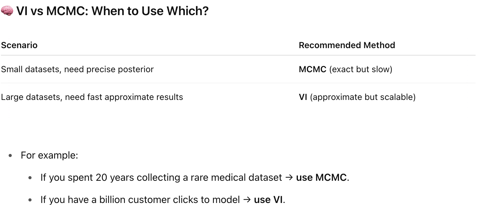
VI vs MCMC: When to Use Which?

Pros and Cons of VI

• Pros:

  • Much faster than MCMC.
  • Easy to scale with stochastic optimization and distributed computation.

• Cons:

  • VI underestimates posterior variance (it tends to be “overconfident”).
  • It does not guarantee exact samples from the true posterior.

Variational Inference

Recall that in the Bayesian framework, $$p(z \mid x) = \frac{p(z,x)}{p(x)} \propto p(x \mid z) p(z)$$ We try to avoid calculating the denominator (marginal likelihood), $p(x)$, also called evidence, as it requires us to calculate high dimensional integrals.

Variational inference turns Bayesian inference into an optimization problem by minimizing KL divergence within a simpler family of distributions, typically using coordinate ascent to maximize the evidence lower bound (ELBO).

First, the optimization goal is

$$ q^*(\mathbf{z})=\underset{q(\mathbf{z}) \in \mathcal{Q}}{\arg \min } KL(q(\mathbf{z}) | p(\mathbf{z} \mid \mathbf{x})), $$

where $q^*$ is the best approximation.

$$ \begin{aligned} KL(q(\boldsymbol{z}) \| p(\boldsymbol{z} \mid \boldsymbol{x})) & =\int_z q(\boldsymbol{z}) \log \left[\frac{q(\boldsymbol{z})}{p(\boldsymbol{z} \mid \boldsymbol{x})}\right] d \boldsymbol{z} \\ & =\int_{\boldsymbol{z}}[q(\boldsymbol{z}) \log q(\boldsymbol{z})] d \boldsymbol{z}-\int_{\boldsymbol{z}}[q(\boldsymbol{z}) \log p(\boldsymbol{z} \mid \boldsymbol{x})] d \boldsymbol{z} \\ & =\mathbb{E}_q[\log q(\boldsymbol{z})]-\mathbb{E}_q[\log p(\boldsymbol{z} \mid \boldsymbol{x})] \\ & =\mathbb{E}_q[\log q(\boldsymbol{z})]-\mathbb{E}_q\left[\log \left[\frac{p(\boldsymbol{x}, \boldsymbol{z})}{p(\boldsymbol{x})}\right]\right] \\ & =\mathbb{E}_q[\log q(\boldsymbol{z})]-\mathbb{E}_q[\log p(\boldsymbol{x}, \boldsymbol{z})]+\mathbb{E}_q[\log p(\boldsymbol{x})] \\ & =\mathbb{E}_q[\log q(\boldsymbol{z})]-\mathbb{E}_q[\log p(\boldsymbol{x}, \boldsymbol{z})]+\log p(\boldsymbol{x}) \end{aligned} $$

Note that, $\log p(\boldsymbol{x})$ does not contain $q(\cdot)$, so we can ignore it in the optimization. We define evidence lower bound (ELBO) as

$$ \operatorname{ELBO}(q)=\mathbb{E}_q[\log p(\boldsymbol{x}, \boldsymbol{z})]-\mathbb{E}_q[\log q(\boldsymbol{z})] $$

This value is called evidence lower bound because it is the lower bound of “log evidence”.

$$ \begin{aligned} \log p(\boldsymbol{x}) & =\operatorname{ELBO}(q)+KL(q(\boldsymbol{z}) \| p(\boldsymbol{z} \mid \boldsymbol{x})) \\ & \geq \operatorname{ELBO}(q) \end{aligned} $$

The second line holds because $KL(\cdot | \cdot) \ge 0$ by Jensen’s inequality.

Therefore, maximizing ELBO is equivalent to minimizing KL divergence.

$$ \begin{aligned} q^*(\boldsymbol{z}) & =\underset{q(\boldsymbol{z}) \in \mathcal{Q}}{\operatorname{argmin}} KL(q(\boldsymbol{z}) \| p(\boldsymbol{z} \mid \boldsymbol{x})) \\ & =\underset{q(\boldsymbol{z}) \in \mathcal{Q}}{\operatorname{argmax}} \operatorname{ELBO}(\mathrm{q}) \\ & =\underset{q(\boldsymbol{z}) \in \mathcal{Q}}{\operatorname{argmax}}\left\{\mathbb{E}_q[\log p(\boldsymbol{x}, \boldsymbol{z})]-\mathbb{E}_q[\log q(\boldsymbol{z})]\right\} \end{aligned} $$

What is the intuition for $\operatorname{ELBO}(q)$?

$$ \begin{aligned} \operatorname{ELBO}(q) & \triangleq \mathbb{E}_q[\log p(\boldsymbol{x}, \boldsymbol{z})]-\mathbb{E}_q[\log q(\boldsymbol{z})] \\ & =\mathbb{E}[\log p(\mathbf{z})]+\mathbb{E}[\log p(\mathbf{x} \mid \mathbf{z})]-\mathbb{E}[\log q(\mathbf{z})] \\ & =\mathbb{E}[\log p(\mathbf{x} \mid \mathbf{z})]-\mathrm{KL}(q(\mathbf{z}) \| p(\mathbf{z})) . \end{aligned} $$

• first term is try to “maximize the likelihood”

• second term is try to encourage density $q(\cdot)$ close to prior

• balance between likelihood and prior

Mean-Field Variational Family

In mean field variational inference, we assume that the variational family factorizes,

$$ q(z_1, \cdots, z_m) = \prod_{j=1}^m q_j(z_j), $$ Each variable is independent.

Coordinate ascent algorithm

We will use coordinate ascent inference, iteratively optimizing each variational distribution holding the others fixed.

The ELBO converges to a local minimum. Use the resulting $q$ is as a proxy for the true posterior.

There is a strong relationship between this algorithm and Gibbs sampling.

• In Gibbs sampling we sample from the conditional

• In coordinate ascent variational inference, we iteratively set each factor to

$$ \text{distribution of } z_k \propto \exp {\mathbb{E}[\log(\text{conditional})]} $$

Reference

• Blei, D. M., Kucukelbir ,Alp, & and McAuliffe, J. D. (2017). Variational Inference: A Review for Statisticians. Journal of the American Statistical Association, 112(518), 859–877. https://doi.org/10.1080/01621459.2017.1285773

• Looking for a nice summary? Check this first: Variational Inference - Princeton CS tutorial

• For derivation details, check this: Introduction to Variational Inference