Notes on Instrumental Variables
Here are my notes on instrumental variables from Stefan’s lecture materials.
Motivation
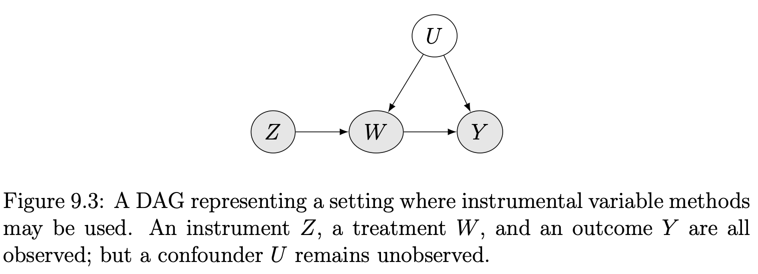
How can we identify causal effects $W \rightarrow Y$ when we are in the presence of unobserved confounding $U$?
One popular way is to find and use instrumental variables.
Partially Linear IV Models
When instrumental variables are available, it becomes possible to point identify causal effects in partially linear models and certain types of causal effects in nonlinear models.
Here we begin with partially linear models.
This is a semiparametric specification, in that we impose a linear relationship between $W$ and $Y$ but let the rest be non-parametric. Notice that, besides the linearity assumption, we also assume a constant treatment effect (i.e. $\tau$), which is also a strong assumption.
When the constant treatment effect model (PLM) doesn’t hold, the average treatment effect $\tau_{ATE} = \E [Y_i (1) − Y_i (0)]$ is NOT identified without more data, because we don’t have any observations on treated never takers, etc. Without linearity, the estimator $\tau_{IV}$ still converges to a large-sample limit $\tau_{LATE}$, the local average treatment effect (LATE).
Identifying assumptions
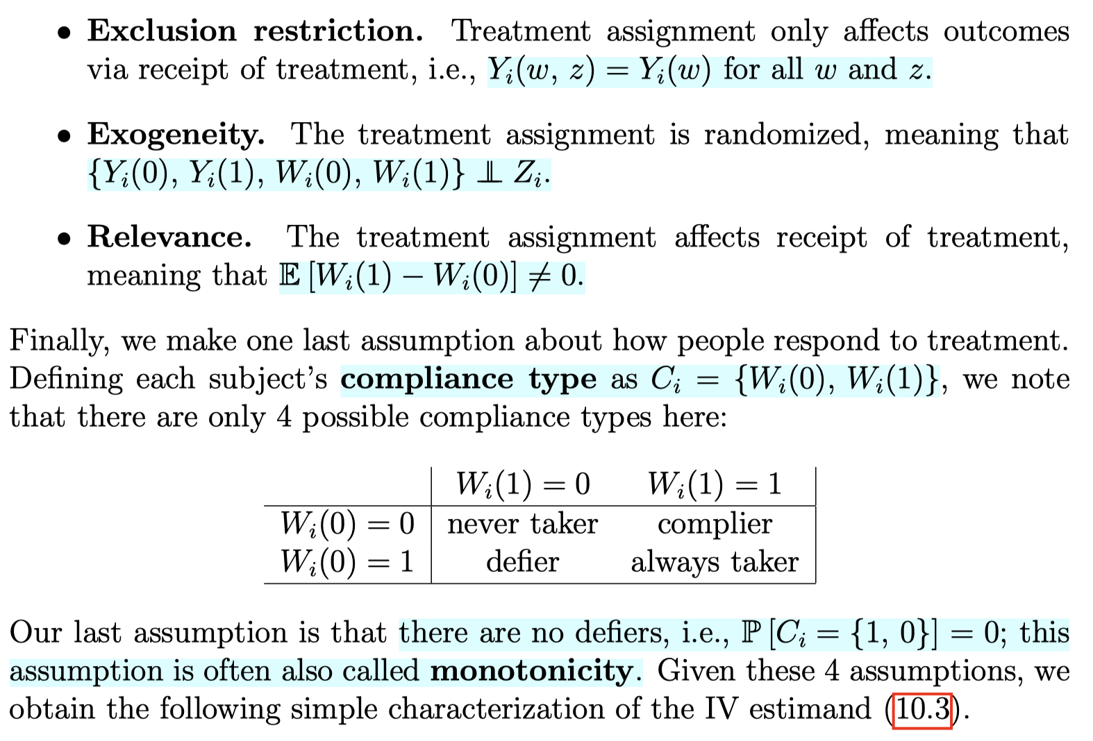
There are 3 identification assumptions. Or let’s say there are three main assumptions that must be satisfied for a variable $Z$ to be considered an instrument.
Graphically, the relevance assumption corresponds to the existence of an active edge from $Z$ to $W$ in the causal graph.
Graphically, this means that we’ve excluded enough potential edges between variables in the causal graph so that all causal paths from $Z$ to $Y$ go through $W$.
Case I (Easiest)
Consider the fully linear version,
$$ \begin{align} & Y=\alpha+W \tau+\varepsilon, \quad \varepsilon \indep Z \tag{C1} \\ & W=Z \gamma+\eta \end{align} $$Then,
$$\operatorname{Cov}[Y, Z]=\operatorname{Cov}[\tau W+\varepsilon, Z]=\tau \operatorname{Cov}[W, Z] $$ $$\tau= \frac{\operatorname{Cov}[Y, Z]}{\operatorname{Cov}[W, Z]}$$It implies,
$$ \hat{\tau}_{IV}= \frac{\widehat{\operatorname{Cov}}[Y_i, Z_i]}{\widehat{\operatorname{Cov}}[W_i, Z_i]} $$
Case II (More general: optimal instruments)
Case I assumes (1) linear relationship between $Y$ and $W$ and (2) linear relationship between $W$ and $Z$. This may be too restrictive. How to extend to more general specification? What should we do if
-
we have multiple instruments
-
or we believe that the instrument may act non-linearly
Consider the following,
$$ Y=\tau W+\varepsilon, \quad \varepsilon \indep Z, \quad Y, W \in \mathbb{R}, \quad Z \in \mathcal{Z}, \tag{C2} $$
where $\mathcal{Z}$ can be a high-dimensional space. Define function $w$ that maps $Z_i$ to the real line $$w: \mathcal{Z} \rightarrow \R$$
Then by the same argument as the Case I (note: we can regard $w(Z)$ as a “pseudo $Z$”),
$$ \tau=\frac{\operatorname{Cov}[Y, w(Z)]}{\operatorname{Cov}[W, w(Z)]} $$
provided the denominator is non-zero, resulting a feasible estimator
$$ \hat{\tau}_{I V}=\frac{\widehat{\operatorname{Cov}}\left[Y_i, w\left(Z_i\right)\right]}{\widehat{\operatorname{Cov}}\left[W_i, w\left(Z_i\right)\right]}=\frac{\frac{1}{n} \sum_{i=1}^n\left(Y_i-\bar{Y}\right)\left(w\left(Z_i\right)-\overline{w(Z)}\right)}{\frac{1}{n} \sum_{i=1}^n\left(W_i-\bar{W}\right)\left(w\left(Z_i\right)-\overline{w(Z)}\right)} $$What is the best function $w$, say $w^*(z)$, that minimizes the variance $V_w$? It turns out that the optimal instrument is the best prediction of $W_i$ from $Z_i$.
$$ w^*(z)=\mathbb{E}\left[W_i \mid Z_i=z\right] $$
How to do we estimate? Do cross-fitting! Why? Because
$$ \epsilon_i \rightarrow W_i \rightarrow \hat{w}(Z_i) $$We no longer have $\hat{w}(Z_i) \indep \epsilon_i$. Therefore, we need cross-fitting to address this issue.
Case III (Much more general: non-parametric IV regression)
The more general version than Case II is the following,
$$ Y_i=\alpha+g\left(W_i\right)+\varepsilon_i, \quad Z_i \indep \varepsilon_i, \quad Y_i, W_i \in \mathbb{R}, \quad Z_i \in \mathcal{Z} \tag{C3} $$
where $g(\cdot)$ is some generic smooth function we want to estimate. Note that:
-
(C3) still requires the effect of $W_i$ on $Y_i$ to be additive
-
however, unlike (C2), it now allows this additive effect to be modified by a non-linearity $g(\cdot)$
Now,
$$ \begin{aligned} \mathbb{E}\left[Y_i \mid Z_i=z\right] & =\mathbb{E}\left[\alpha+g\left(W_i\right)+\varepsilon_i \mid Z_i=z\right] \\ & =\alpha+\mathbb{E}\left[g\left(W_i\right) \mid Z_i=z\right] \\ & =\alpha+\int_{\mathbb{R}} g(w) f(w \mid z) d w, \end{aligned} $$There are two steps for learning $g(\cdot)$:
-
non-parametric model $\hat{f}(w \mid z)$ using cross-fitting
-
estimate $g(\cdot)$ using empirical minimization
For more details, see Section 9.2 in Stefan’s lecture.
Local Average Treatment Effects
Motivation
-
IV without the linearity assumption: One may doubt the validity the linearity and constant treatment effect assumption in previous section. What about non-parametric identification using IV?
-
Encouragement Design and Noncompliance: Noncompliance is a common problem in encouragement designs involving human beings as experimental units. In those cases, the experimenters cannot force the units to take the treatment but rather only encourage them to do so. Heterogeneous effects should be allowed.
Setup
Consider an randomized experiment,
-
Let $Z_i \in \{0, 1\}$ be the treatment assigned
-
Let $W_i \in \{0, 1\}$ be the treatment received
-
When $Z_i \neq W_i$, the noncompliance problem arises
-
Potential outcome $\{W_i(1), W_i(0)\}$ s.t. $W_i = W_i(Z_i)$
-
Potential outcome $\{Y_i(w,z)\}_{(w,z) \in \{0,1\}}$ s.t. $Y_i = Y_i(W_i, Z_i)$
Identifying assumptions
LATE Theorem
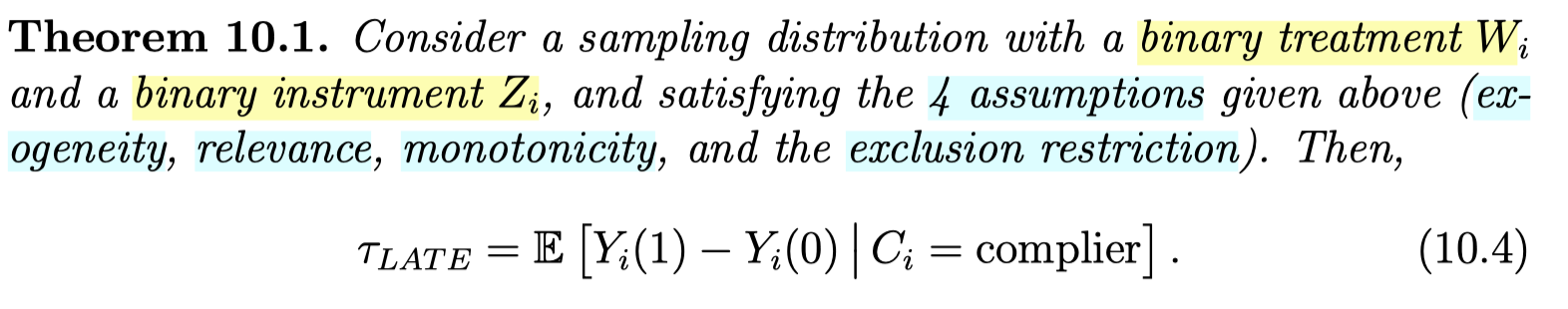
Idea of proof:
-
Start with $\Cov(Y, Z) = \E[YZ] - \E[Y]\E[Z]$, then apply LIE by conditioning on $Z$
-
Derive $\Cov(W, Z)$ similarly as above, then get the ratio
-
Decompose the ATE on $Y$, $\E[Y(1) - Y(0)]$, into four terms (always-taker, compiler, defier, never-taker) using law of total probability
-
By exclusion restriction and monotonicity assumption, only “compiler” remains
Multiple instruments
We may have access to data from multiple randomized trials that can be used to study a treatment effect via a non-compliance analysis.
Marketing example:
-
goal: study the effect of subscription to a loyalty program ($W_i$) on long-term customer CLV ($Y_i$)
-
randomized trial 1: offering discounts for joining the loyalty program $\left(Z_i=\1(\{\right.$ customer received a discount $\left.\})\right)$
-
randomized trial 2: showing advertisements $\left(Z_i=\1(\{\right.$ customer was shown an ad for the program $\left.\})\right)$
Previously, under the linear treatment effect model, multiple instruments could be combined into a single optimal instrument, and the optimal instrument corresponds to the summary of all the instruments that best predicts the treatment.
Without the linear treatment effect model, however, we caution that no such result is available. Different instruments may induce difference compliance patterns, and so the LATEs identified different instruments may not be the same.
In the marketing example, the ATE for customers who respond to a discount may be different from the ATE for customers who respond to an advertisement.
Reference
Wager, S. (2024). Causal inference: A statistical learning approach. https://web.stanford.edu/~swager/causal_inf_book.pdf