Notes on Matrix Completion Methods

Jul 8, 2025 11 min read causal inference

Here are my study notes on the matrix completion method for causal panel data models proposed by Athey et al. (2021).

1. Setup and Notation

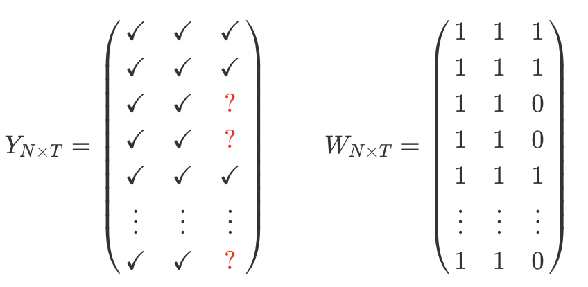
Let $Y (0), Y (1)$ be potential outcome matrices, $W$ be a matrix of binary treatment, $W_{i t} \in {0, 1}$ .

Rows ( $i$ ) of $Y$ and $W$ correspond to units
Columns ( $t$ ) of $Y$ and $W$ correspond to time periods

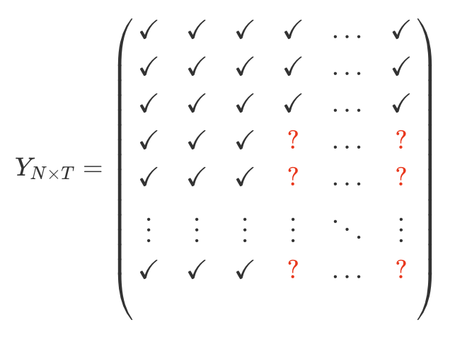
We would need to impute the missing potential outcomes in $Y (0)$ , a $N \times T$ matrix, denoted as $Y_{N \times T}$ .

From now on, I drop from here on the $(0)$ part of $Y (0)$
I will simply use $Y$ to refer to $Y (0)$

This is now a matrix completion problem.

For illustration, let’s consider the structure on the missing data to be block structure, with a subset of the units adopting an irreversible treatment at a particular point in time $T_{0} + 1$ . Note that this method can also handle the staggered treatment case.

Let $M$ denote the set of pairs of indices $(i, t) \in [N] \times [T]$ , corresponding to the missing entries. Let $O$ denote the set of pairs of indices corresponding to the observed entries.

The causal parameter of interest is the treatment effect on treated (ATT). $τ = \frac{\sum_{i, t} W_{i t} (Y_{i t} (1) - Y_{i t} (0))}{\sum_{i t} W_{i t}}$

2. Horizontal / Unconfoundedness Regression

The unconfoundedness literature focuses on:

The single-treated-period structure with a thin matrix $(N ≫ T)$ .
A large number of treated and control units

Impute the missing potential outcomes using control units with similar lagged outcomes

Remark 1.

Does it remind you time series forecasting with exponential smoothing – more recent observations have higher weights, while more distant ones have lower weights. However, the horizontal regression approach uses linear regression on lagged observations to choose weights.

In this setting, the identification depends on the following assumption.

Assumption 1 (Identification Assumption).

For the units with

(i, t) \in M

, i.e., the units that have missing entries,

Y_{i, T} (0) ⊥ ⊥ W_{i, T} ∣ Y_{i, 1}, \dots, Y_{i, T - 1},

Roughly speaking, the idea is that if conditional on the pre-treatment outcomes, the treatment assignment is as good as random, then we can use flexible control methods (e.g. doubly robust method).

The horizontal or unconfoundedness type of regression is to regress the last period outcome on the lagged outcomes and use the estimated regression to predict the missing potential outcomes.

$lm (Y_{i T} \sim 1 + Y_{i 1} + Y_{i 2} + \dots + Y_{i, T - 1})$
Predict ${\hat{Y}}_{i T}$ using the linear combination of its historical observations

For the units with $(i, t) \in M$ , the predicted outcome is:

${\hat{Y}}_{i T} = {\hat{β}}_{0} + \sum_{s = 1}^{T - 1} {\hat{β}}_{s} Y_{i s},$ where

\hat{β} = \arg min_{β} \sum_{i : (i, T) \in O} {(Y_{i T} - β_{0} - \sum_{s = 1}^{T - 1} β_{s} Y_{i s})}^{2} .

Assumption 2 (Patterns over time are stable across units).

Horizontal / unconfoundedness approach assumes that patterns over time are stable across units.

More specifically, it assumes there is relation between outcomes in treated period and pre-treatment periods that is the same for all units. Note:

β_{s}

is the same for ALL units

i

A more flexible, nonparametric, version of this estimator would correspond to matching,

For each treated unit $i$ , we find a corresponding control unit $j$ with $Y_{j t} \approx Y_{i t}$ for all pre-treatment periods $t = 1, \dots, T - 1$ .

If $N$ is large relative to $T_{0}$ , use regularized regression such as LASSO, Ridge, and Elastic Net.

3. Vertical Regression and the Synthetic Control literature

The synthetic control methods focus on:

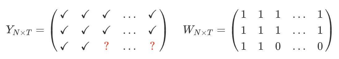
The single-treated-unit block structure with a fat $(T ≫ N)$ or approximately square $(T \approx N)$ matrix.
A large number of pre-treatment periods (i.e. $T_{0}$ is large)
$Y_{N t}$ is missing for $t \geq T_{0}$ and there are no missing entries for other units

vertical-regression-matrix — Figure 3: fat matrix

In this setting, the identification depends on the assumption that:

Assumption 3 (Identification Assumption).

Y_{N, t} (0) ⊥ ⊥ W_{N, T} ∣ Y_{1, t}, \dots, Y_{N - 1, T}

Previous studies¹ show how the synthetic control method can be interpreted as regressing the outcomes for the treated unit prior to the treatment on the outcomes for the control units in the same periods.

$lm (Y_{N, t} \sim 1 + Y_{1 t} + Y_{2 t} + \dots + Y_{N - 1, t})$ , for $t = T_{0}, \dots, T$

That is, for the treated unit in period $t$ , for $t = T_{0}, \dots, T$ , the predicted outcome is:

{\hat{Y}}_{N t} = {\hat{ω}}_{0} + \sum_{i = 1}^{N - 1} {\hat{ω}}_{i} Y_{i t}

where

\hat{ω} = \arg min_{ω} \sum_{t : (N, t) \in O} {(Y_{N t} - ω_{0} - \sum_{i = 1}^{N - 1} ω_{i} Y_{i s})}^{2} .

This is referred to as vertical regression.

Assumption 4 (Patterns across units are stable over time).

Vertical / synthetic control approach assumes that patterns across units are stable over time.

More specifically, it assumes there is relation between different units that is stabale over time. Note:

ω_{i}

is the same for ALL time period

t

A more flexible, nonparametric, version of this estimator would correspond to matching,

For each post-treatment period $t$ we find a corresponding pre-treatment period $s$ with $Y_{i s} \approx Y_{i t}$ for all control units $i = 1, \dots, N - 1$ .

If $T$ is large relative to $N_{c}$ , one could use regularized regression such as LASSO, Ridge, and Elastic Net.

4. Panel with Fixed Effects

Before move to fixed effect, factor and interactive mixed effect models, let’s do a short summary.

Horizontal regression:

Data: Thin matrix (many units, few periods), single treated period (period $T$ )
Strategy: Use controls to regress $Y_{i T}$ on lagged outcomes $Y_{i 1}, Y_{i 2}, \dots, Y_{i, T - 1}$
- $lm (Y_{i T} \sim 1 + Y_{i 1} + Y_{i 2} + \dots + Y_{i, T - 1})$
- $N_{C}$ observations, $T - 1$ regressors
Does not work well if $Y$ is fat (few units, many periods)
Key identifying assumption: $Y_{i, T} (0) ⊥ ⊥ W_{i, T} ∣ Y_{i, 1}, \dots, Y_{i, T - 1}$

The horizontal regression focuses on a pattern in the time path of the outcome $Y_{i t}$ , specifically the relation between $Y_{i T}$ and the lagged $Y_{i t}$ for $t = 1, \dots, T - 1$ for the units for whom these values are observed, and assumes that this pattern is the same for units with missing outcomes.

Vertical regression

Data: Fat matrix (few units, many periods), single treated unit (unit $N$ ), treatment starts in period $T_{0}$ .
Strategy: Use pretreatment periods to regress $Y_{N, t}$ on contemporaneous outcomes $Y_{1 t}, Y_{2 t}, \dots, Y_{N - 1, t}$
- $lm (Y_{N, t} \sim 1 + Y_{1 t} + Y_{2 t} + \dots + Y_{N - 1, t})$
- $T_{0} - 1$ observations, $N$ regressors
Does not work well if matrix is thin (many units)
Key identifying assumption: $Y_{N, t} (0) ⊥ ⊥ W_{N, T} ∣ Y_{1, t}, \dots, Y_{N - 1, T}$

The vertical regression focuses on a pattern between units at times when we observe all outcomes, and assumes this pattern continues to hold for periods when some outcomes are missing.

However, by focusing on only one of these patterns, cross-section or time series, these approaches ignore alternative patterns that may help in imputing the missing values. One alternative is to consider approaches that allow for the exploitation of stable patterns over time and stable patterns across units. Such methods have a long history in panel data literature, including the two-way fixed effects, and factor and interactive mixed effect models.

In the absence of covariates, the common two-way fixed effect model is:

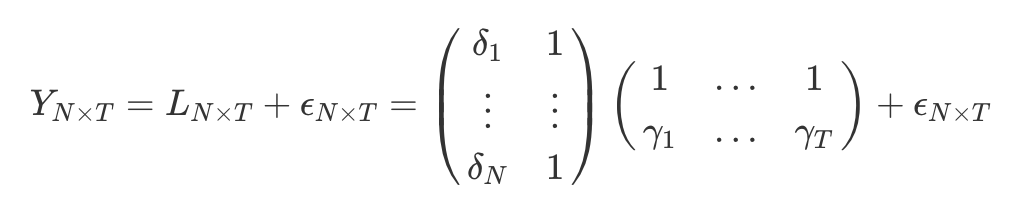
Y_{i t} = δ_{i} + γ_{t} + ϵ_{i t}

In this setting, the identification depends on the assumption that:

Y_{i, t} (0) ⊥ ⊥ W_{i, T} ∣ δ_{i}, γ_{t} .

So the predicted outcome based on the unit and time fixed effects is:

{\hat{y}}_{N T} = {\hat{δ}}_{N} + {\hat{γ}}_{T}

In a matrix form, the model can be rewritten as:

The matrix formulation of the identification assumption is:

Y_{N \times T} (0) ⊥ ⊥ W_{N \times T} ∣ L_{N \times T}

5. Interactive Fixed Effects

5.1 Why Use Interactive Fixed Effects?

In panel data, traditional fixed effects control for differences across units and time periods. But what if there are hidden factors that evolve over time and affect each unit differently — like how each state reacts differently to national economic trends?

Classical models can’t handle that. This is where interactive fixed effects shine: they model these latent time-varying confounders using a flexible structure, $λ_{i}^{'} F_{t}$ (Bai 2009), helping us avoid bias when estimating causal effects.

5.2 Interactive Fixed Effects Model

For interactive fixed effects, instead of exploiting additive structure in unit and time effects, we exploit the low rank or interactive structure of unit and time fixed effects for panel data regression.

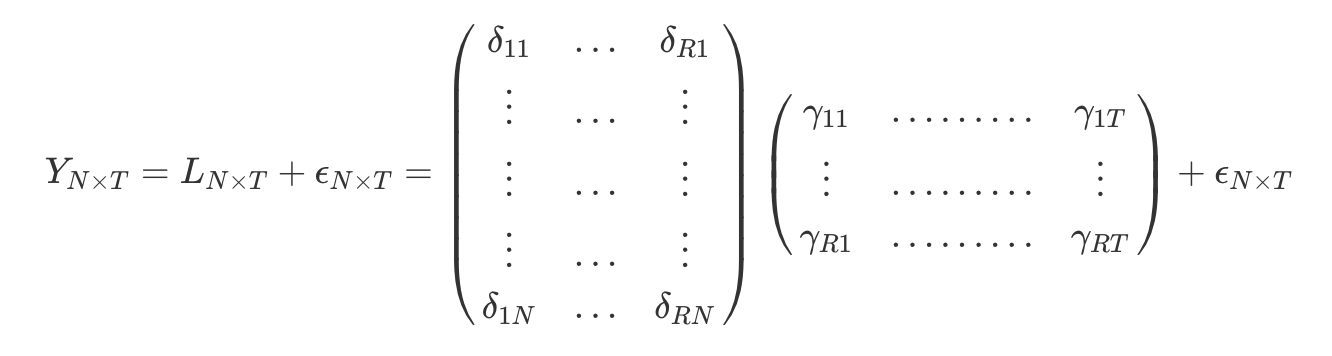
The common interactive fixed effect model is:

Y_{i t} = \sum_{r = 1}^{R} δ_{i r} γ_{t r} + ε_{i t},

where

$γ_{t r}$ are called factors
- Note: Factors are unobserved, time-varying variables that capture common influences or shocks affecting all units at time $t$ . They represent the latent drivers of the outcome that change over time but are shared across units.
$δ_{i r}$ are called factor loadings
- Note: Factor loadings are unobserved, unit-specific coefficients that determine how much each unit $i$ is affected by the common factors. They reflect the heterogeneity in how units respond to the time-varying factors.

Note that both factors and factor loadings are parameters that need to be estimated. Typically it is assumed that the number of factors $R$ is fixed, although it is not necessarily known to the researcher.

Again, the identification depends on the assumption that:

$Y_{i, t} (0) ⊥ ⊥ W_{i, T} ∣ δ_{i}, γ_{t} .$

The predicted outcome based on the interactive fixed effects would be:

{\hat{y}}_{N T} = \sum_{r = 1}^{R} {\hat{δ}}_{i r} {\hat{γ}}_{t r}

In a matrix form, the $Y_{N \times T}$ can be rewritten as:

The matrix formulation of the identification assumption is:

Y_{N \times T} (0) ⊥ ⊥ W_{N \times T} ∣ L_{N \times T}

Using the interactive fixed effects model, we would estimate $δ$ and $γ$ by least squares regression and use those to impute missing values.

6. The Matrix Completion with Nuclear Norm Minimization Estimator

In the absence of covariates, the $Y_{N \times T}$ matrix can be rewritten as

Y_{N \times T} = L_{N \times T} + ϵ_{N \times T}

Assumption 5 (Key assumptions).

W_{N \times T} ⊥ ⊥ ε_{N \times T}

(but

W

may depend on

L

).
2. There exists staggered entry relating to the weights such that

W_{i t + 1} \geq W_{i t}

L

has a low rank relative to

N

and

T

In a more general case, Y_{i t}$ is equal to:

Y_{i t} = L_{i t} + \sum_{p = 1}^{P} \sum_{q = 1}^{Q} X_{i p} H_{p q} Z_{q t} + γ_{i} + δ_{t} + V_{i t} β + ε_{i t}

where

$X_{i}$ : unit-specific $P$ -component covariate
$Z_{t}$ : time-specific $Q$ -component covariate
$V_{i t}$ : unit-time-specific covariate
$γ_{i}$ : unit fixed effect
$δ_{t}$ : time fixed effect

We do not necessarily need the fixed effects $γ_{i}$ and $δ_{t}$ as these can be subsumed into $L$ . However, it is convenient and efficient to include the fixed effects given that we regularize $L$ .

With too many parameters, especially for $N \times T$ matrix $L$ , we need regularization such that we shrink $L$ and $H$ toward zero. To regularize H , we use Lasso-type element-wise $ℓ_{1}$ norm, defined as

‖ H ‖_{1, e} = \sum_{p = 1}^{P} \sum_{q = 1}^{Q} | H_{p q} |

But how do we regularize $L$ ?

By singular value decomposition (SVD), we have $L_{N \times T}$ is equal to:

L_{N \times T} = S_{N \times N} Σ_{N \times T} R_{T \times T}

where

$S, R$ unitary
$Σ$ is rectangular diagonal with entries $σ_{i} (L)$ that are the singular values
Rank of $L$ is number of non-zero $σ_{i} (L)$ .

There are three ways to regularize $L$ :

\begin{aligned} ‖ L ‖_{F}^{2} = \sum_{i, t} {| L_{i t} |}^{2} = \sum_{j = 1}^{min (N, T)} σ_{i}^{2} (L) (Frobenius, like ridge) \\ ‖ L ‖_{*} = \sum_{j = 1}^{mis (N, T)} σ_{i} (L) (nuclear norm, like LASSO) \\ ‖ L ‖_{R} = \sum_{j = 1}^{min (N, T)} 1_{σ_{i} (L) > 0} (Rank, like subset selection) \end{aligned}

Frobenius norm imputes missing values as 0
Rank norm is computationally not feasible for general missing data patterns
The preferred Nuclear norm leads to low-rank matrix and is computationally feasible.

So the Matrix-Completion with Nuclear Norm Minimization (MC-NNM) estimator uses the nuclear norm:

min_{L} \frac{1}{| O |} \sum_{(i, t) \in 0} {(Y_{i t} - L_{i t})}^{2} + λ_{L} ‖ L ‖_{*}

For the general case, we estimate $H, L, δ, γ$ , and $β$ as

min_{H, L, δ, γ} \frac{1}{| O |} \sum_{(i, t) \in O} {(Y_{i t} - L_{i t} - \sum_{p = 1}^{P} \sum_{q = 1}^{Q} X_{i p} H_{p q} Z_{q t} - γ_{i} - δ_{t} - V_{i t} β)}^{2} + λ_{L} ‖ L ‖_{*} + λ_{H} ‖ H ‖_{1, e}

And we choose $λ_{L}$ and $λ_{H}$ through cross-validation.

Reference

Athey, Susan, Mohsen Bayati, Nikolay Doudchenko, Guido Imbens, and Khashayar Khosravi (2021), “Matrix Completion Methods for Causal Panel Data Models,” Journal of the American Statistical Association, 116 (536), 1716–30.

Liu, Licheng, Ye Wang, and Yiqing Xu (2024), “A Practical Guide to Counterfactual Estimators for Causal Inference with Time-Series Cross-Sectional Data,” American Journal of Political Science, 68 (1), 160–76.

Chapter 8 Matrix Completion Methods | Machine Learning-Based Causal Inference Tutorial

7.1 Simple Exponential Smoothing | Forecasting: Principles And Practice (2nd Ed)

Bai, Jushan (2009), “Panel Data Models With Interactive Fixed Effects,” Econometrica, 77 (4), 1229–79.

R packages 📦 to implement: