Notes on Propensity Score Methods

Jun 3, 2025 6 min read causal inference, econometrics

$$ \newcommand{\indep}{\mathrel{\perp\mkern-10mu\perp}} \newcommand{\P}{\mathbb{P}} \newcommand{\R}{\mathbb{R}} \newcommand{\E}{\mathbb{E}} \newcommand{\Var}{\operatorname{Var}} \newcommand{\Cov}{\operatorname{Cov}} \newcommand{\1}[1]{\mathbf{1}\\{#1\\}} $$

Introduction

Here are my notes on propensity scores, mainly from Prof. Ding’s textbook (2024).

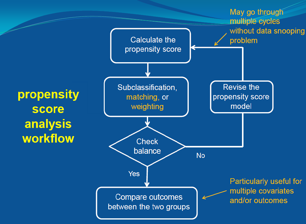
The traditional propensity score analysis workflow is shown in the image below, which I will not cover in detail. Instead, I will summarize the key theorems and results from Ding’s textbook.

Image from Chap3.3_observational_PS, page 16 — Figure 1: Traditional propensity score analysis workflow

I will also provide some connections with Riesz Representer (RR).

Why connect with the Riesz Representer (RR)? The connection provides a powerful generalization of the foundational Rosenbaum-Rubin (1983) result.
Rosenbaum and Rubin showed that conditioning on the propensity score is sufficient for removing confounding bias when estimating causal effects. The Riesz representer extends this principle: it suffices to regress on the Riesz representer to obtain unbiased estimates of the average treatment effect.
The key insight is that the Riesz representer, like the propensity score, serves as a sufficient statistic – it captures all the confounding information necessary for unbiased estimation of your target causal parameter.

Setting & Notation

Binary treatment $Z$
Potential outcomes $\{Y(0), Y(1)\}$
Propensity score: $\P(Z = 1 \mid X)$, where $X$ represents covariates

Two approaches learning causal relationships:

Outcome process (via outcome regression)
Treatment assignment mechanism (via propensity score)

The following summarizes the key theorems and results related to propensity scores from Prof. Ding’s textbook.

1. The propensity score as a dimension reduction tool

Theorem 1 (pscore as dimension reduction tool).

$$ \text { If } Z \indep \{Y(1), Y(0)\} \mid X, \text { then } Z \indep \{Y(1), Y(0)\} \mid e(X) . $$

Covariates $X$ can be high dimensional, but the propensity score, $e(X) \in \R$, is a 1-dimensional scalar
We can view the propensity score as a dimensional reduction tool

2. Propensity score stratification

Idea: Discretize the estimated propensity score by its $K$ quantiles:
$$ Z \indep \{Y(1), Y(0)\} \mid \hat{e}^{\prime}(X)=e_k \quad(k=1, \ldots, K) . $$
Estimate ATE within each subclass and then average by the block size
Advantage: The propensity score stratification estimator only requires the correct ordering of the estimated propensity scores rather than their exact values, which makes it relatively robust compared with other methods

3. Propensity score weighting

Theorem 2 (Invese propensity score weighting (IPW)).

If $Z \indep \{Y(1), Y(0)\} \mid X$ and $ 0 < e(X) < 1$, then $$E\{Y(1)\}=E\left\{\frac{Z Y}{e(X)}\right\}, \quad E\{Y(0)\}=E\left\{\frac{(1-Z) Y}{1-e(X)}\right\}$$ and $$ \begin{aligned} \tau &=E\{Y(1)-Y(0)\}\\ &=E\left\{\frac{Z Y}{e(X)}-\frac{(1-Z) Y}{1-e(X)}\right\} \\ &=E\left\{HY \right\} \end{aligned} $$ where $H := \left[\frac{Z}{e(X)}-\frac{(1-Z) }{1-e(X)}\right]$ is called the Horvitz-Thompson transform.

Connection the Riesz Representer (RR)

Remark 1 (RR in the case of ATE).

In the case of ATE, the Riesz Representer, $\alpha(Z, X)$, has the same form as above Horvitz-Thompson transform, $$ \alpha(Z, X) = \left[\frac{Z}{e(X)}-\frac{(1-Z) }{1-e(X)}\right] $$

3.1 Estimation

The sample version of IPW is called the Horvitz–Thompson (HT) estimator,
$$ \hat{\tau}^{\mathrm{ht}}=\frac{1}{n} \sum_{i=1}^n \frac{Z_i Y_i}{\hat{e}\left(X_i\right)}-\frac{1}{n} \sum_{i=1}^n \frac{\left(1-Z_i\right) Y_i}{1-\hat{e}\left(X_i\right)} $$
HT estimator $\hat{\tau}^{\mathrm{ht}}$ has many problems
Problem: lack of invariance, i.e. if we replace $Y_i$ by $Y_i + c$, $\hat{\tau}^{\mathrm{ht}}$ changed because it depends on $c$. This is not reasonable.
Solution: normalizing the weights
$$ \hat{\tau}^{\text {hajek }}=\frac{\sum_{i=1}^n \frac{Z_i Y_i}{\hat{e}\left(X_i\right)}}{\sum_{i=1}^n \frac{Z_i}{\hat{e}\left(X_i\right)}}-\frac{\sum_{i=1}^n \frac{\left(1-Z_i\right) Y_i}{1-\hat{e}\left(X_i\right)}}{\sum_{i=1}^n \frac{1-Z_i}{1-\hat{e}\left(X_i\right)}} . $$
Hajek estimator is invariant to the location transformation

3.2 Strong overlap condition

Many asymptotic analyses require a strong overlap condition,

$$ 0<\alpha_{\mathrm{L}} \leq e(X) \leq \alpha_{\mathrm{U}}<1 $$ In practice,

Crump et al. (2009) suggested $α_L = 0.1$ and $α_U = 0.9$
Kurth et al. (2005) suggested $α_L = 0.05$ and $α_U = 0.95$

4. Balancing property

Theorem 3 (balancing property).

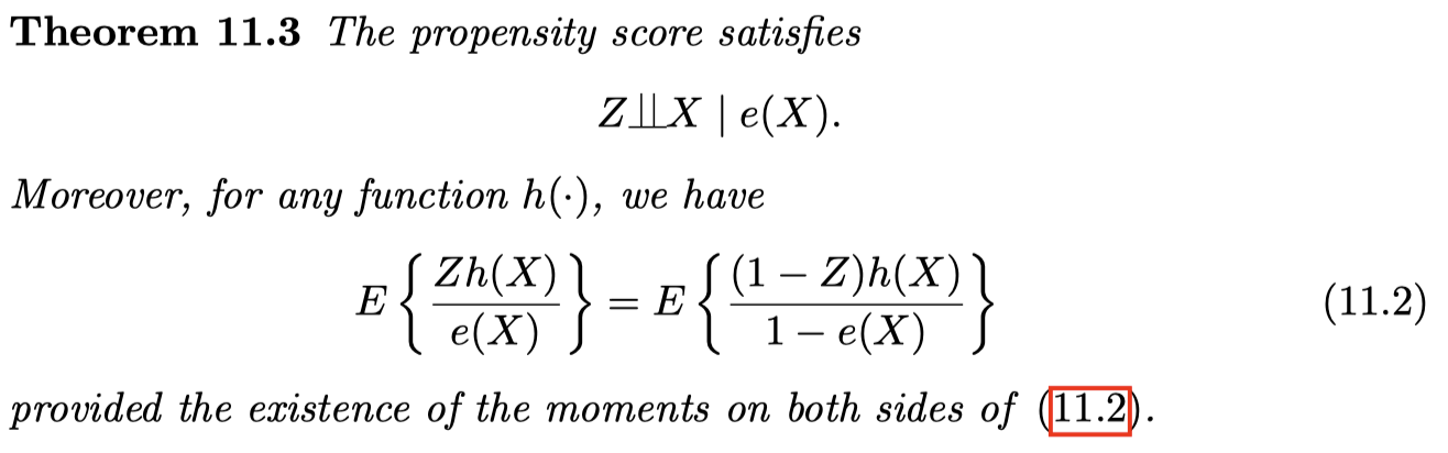
Conditional on $e(X)$, the treatment and the covariates are independent
Within the same level of the propensity score, the covariate distributions are balanced across the treatment and control groups
Useful implication: we can check whether the propensity score model is specified well enough to ensure the covariate balance in the data

4.1 Propensity score is a balancing score

Definition 1.

Theorem 4 (Propensity score is a balancing score).

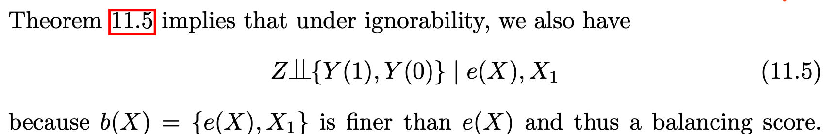
This is relevant in subgroup analysis
The conditional independence in (11.5) ensures unconfoundedness holds given the propensity score, within each level of $X_1$. Therefore, we can perform the same analysis based on the propensity score, within each level of $X_1$, yielding estimates for two subgroup effects

5. Doubly Robust or AIPW

The following Theorem is summarized from Prof. Wager’s lecture notes (2024).

Theorem 5 (strong double robustness of AIPW estimator).

Define the outcome regression as $$ \mu_{(z)}(x)=\mathbb{E}\left[Y_i(z) \mid X_i=x\right], $$ Define AIPW estimator as $$ \begin{aligned} \hat{\tau}_{A I P W} & =\underbrace{\frac{1}{n} \sum_{i=1}\left(\hat{\mu}_{(1)}\left(X_i\right)-\hat{\mu}_{(0)}\left(X_i\right)\right)}_{\text { outcome regression estimator }} \\ & +\underbrace{\frac{1}{n} \sum_{i=1}^n\left(\frac{Z_i}{\hat{e}\left(X_i\right)}\left(Y_i-\hat{\mu}_{(1)}\left(X_i\right)\right)-\frac{1-Z_i}{1-\hat{e}\left(X_i\right)}\left(Y_i-\hat{\mu}_{(0)}\left(X_i\right)\right)\right)}_{\text { applying IPW to the regression residuals }} \end{aligned} $$ If we use estimators $\hat{\mu}_{(z)}(x)$ and $\hat{e}(x)$ that are both consistent with root-mean squared error (RMSE) decaying faster than $n^{-\alpha_\mu}$ and $n^{-\alpha_e}$ respectively, and if furthermore $\alpha_\mu+\alpha_e \geq 1 / 2$, then $$ \begin{aligned} & \sqrt{n}\left(\hat{\tau}_{A I P W}-\tau\right) \Rightarrow \mathcal{N}\left(0, V_{A I P W}\right) \\ & V_{A I P W}=\operatorname{Var}\left[\tau\left(X_i\right)\right]+\mathbb{E}\left[\frac{\sigma_0^2\left(X_i\right)}{1-e\left(X_i\right)}\right]+\mathbb{E}\left[\frac{\sigma_1^2\left(X_i\right)}{e\left(X_i\right)}\right] \end{aligned} $$ where $$ \sigma_{(z)}^2(x)=\operatorname{Var}\left[Y_i(z) \mid X_i=x\right] $$

Check my previous post: Intuition for Doubly Robust Estimator
AIPW provides a natural starting point for understanding Double Machine Learning
Key insight of RR in DML framework: Leverage the Riesz Representer, a “generalized version of propensity score” to “correct the bias”

More general, Li et al. (2018a) gave a unified discussion of the causal estimands in observational studies.

Theorem 6 (Ding (2024), Section 13.4).

Summary Table of common estimands:

This table provides us a good way to understand and remember IPW estimator for ATT
How to remember $\tau^h$? Apply IPW on “pseudo outcome” $Yh(X)$ then divide by $E(h(X))$
When the parameter of interest is ATT, then $$E(h(X)) = E(e(X)) = E(E(Z \mid X)) = E(Z) = \P(Z = 1) = e$$
Use it to better understand IPW for ATT

7. Propensity Score in Regression

PS as a covariate

Theorem 7 (regression with pscore as a covariate).

Under unconfoundedness, the coefficient of $Z$ in the population OLS fit of $$ Y \sim 1+Z + e(X) $$ equals $\tau_{\mathrm{O}}$, $$ \tau_{\mathrm{O}}=\frac{E[e(X)\{1-e(X)\} \tau(X)]}{E[e(X)\{1-e(X)\}]} ,$$ which is the overlap-weighted average treatment effect

Based on above Theorem, we also have:

Corollary 1.

Under unconfoundedness,
1. the coefficient of $Z$ in the population OLS fit of $$ Y \sim 1+Z + e(X) + X $$ also equals $\tau_{\mathrm{O}}$,

2. the coefficient of $Z-e(X)$ in the population OLS fit of $$ Y \sim [Z - e(X)] \quad \text{or} \quad Y \sim 1 + [Z - e(X)] $$ also equals $\tau_{\mathrm{O}}$

PS as a weight

There is a convenient way to obtain $\hat{\tau}^{\text{hajek}}$ based on WLS.

Proposition 1 (convenient to obtain $\hat{\tau}^{\text{hajek}}$ based on WLS).

Need to use bootstrap for standard error
Why does the WLS give a consistent estimator for $\tau$ ?
In RCT with a constant propensity score, we can simply use the coefficient of $Z_i$ in the OLS fit of $Y_i$ on ( $1, Z_i$ ) to estimate $\tau$
In observational studies, we need to deal with the selection bias. The key idea is:
- If we weight the treated units by $\frac{1}{e(X_i)}$ and the control units by $\frac{1}{1-e(X_i)}$, then both treated and control groups can represent the whole population
- Thus, by weighting, we effectively have a pseudo-randomized experiment
- Remark 2 (IPCW).
  
  Inverse Probability of Censoring Weighting (IPCW) follows the same idea — it adjusts for censoring bias by reweighting observations based on their probability of being uncensored.
Consequently, the difference between the weighted means is consistent for $\tau$. The numerical equivalence of $\hat{\tau}^{\text {hajek }}$ and WLS is not only a fun numerical fact itself but also useful for motivating more complex estimators with covariate adjustment

Reference

Ding, Peng (2024), A First Course in Causal Inference, CRC Press.

Wager, S. (2024). Causal inference: A statistical learning approach. https://web.stanford.edu/~swager/causal_inf_book.pdf

propensity score weighting treatment assignment mechanism IPW AIPW Riesz Representer IPCW

Chen Xing

Founder & Data Scientist

Enjoy Life & Enjoy Work!